We test the Multi-Period Optimization model on a real estate portfolio.
This is an example that shows that Cvxportfolio can work as well with
different asset classes. We use the Case-Shiller index as proxy for the price
of housing units in various metropolitan areas in the USA. We impose realistic
transaction costs, which are comparable to the annual return on the asset, and
we show that multi-period optimization is useful to correctly balance
transaction cost and expected risk-adjusted return.
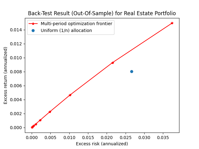
We present the (Cvxportfolio native) plots of the results of various
back-tests, and also create an “efficient frontier” plot obtained by
sweeping over choices of the risk aversion hyper-parameter.
importmatplotlib.pyplotaspltimportnumpyasnpimportcvxportfolioascvx# These are monthly time serieses of the Case-Shiller index for# a selection of US metropolitan areas. You can find them on the# website of FRED https://fred.stlouisfed.org/UNIVERSE=['SFXRSA',# San Francisco'LXXRSA',# Los Angeles'SEXRSA',# Seattle'DAXRSA',# Dallas'SDXRSA',# San Diego'MIXRSA',# Miami'PHXRSA',# Phoenix'NYXRSA',# New York'CHXRSA',# Chicago'ATXRSA',# Atlanta'LVXRSA',# Las Vegas'POXRSA',# Portland'WDXRSA',# Washington D.C.'TPXRSA',# Tampa'CRXRSA',# Charlotte'MNXRSA',# Minneapolis'DEXRSA',# Detroit'CEXRSA',# Cleveland'DNXRSA',# Denver'BOXRSA',# Boston]# we assume that the cost of transacting# residential real estate is about 5%LINEAR_TCOST=0.05simulator=cvx.MarketSimulator(universe=UNIVERSE,# we enabled the default data interface to download index# prices from FREDdatasource='Fred',costs=[cvx.TransactionCost(a=LINEAR_TCOST,b=None,# since we don't have market volumes, we can't use the# market impact term of the transaction cost model)])# let's see what a uniform allocation doesresult_uniform=simulator.backtest(cvx.Uniform())print('BACK-TEST RESULT OF UNIFORM (1/N) ALLOCATION')print(result_uniform)# plot the resultfigure_uniform=result_uniform.plot()# These are risk model coefficients. They don't seem to have# a strong effect on this example.NUM_FACTORS=5KAPPA=0.1# This is the multi-period planning horizon. We plan for 6 months# in the future.HORIZON=6policies=[]# sweep over risk aversionforgamma_riskinnp.logspace(0,3,10):policies.append(cvx.MultiPeriodOptimization(cvx.ReturnsForecast()-gamma_risk*(cvx.FactorModelCovariance(num_factors=NUM_FACTORS)+KAPPA*cvx.RiskForecastError())-cvx.TransactionCost(a=LINEAR_TCOST,b=None),[cvx.LongOnly(applies_to_cash=True)],planning_horizon=HORIZON,))# run parallel back-tests for all the policies defined aboveresults=simulator.backtest_many(policies)print('BACK-TEST RESULT OF MPO WITH HIGHEST (OUT-OF-SAMPLE) PROFIT')print(results[np.argmax([el.profitforelinresults])])# back-test result with the highest profittop_profit_fig=results[np.argmax([el.profitforelinresults])].plot()# multi-period optimization efficient frontierefficient_frontier_figure=plt.figure()plt.plot([result.excess_returns.std()*np.sqrt(12)forresultinresults],[result.excess_returns.mean()*12forresultinresults],'r*-',label='Multi-period optimization frontier')plt.scatter([result_uniform.excess_returns.std()*np.sqrt(12)],[result_uniform.excess_returns.mean()*12],label='Uniform (1/n) allocation')plt.legend()plt.title('Back-Test Result (Out-Of-Sample) for Real Estate Portfolio')plt.xlabel('Excess risk (annualized)')plt.ylabel('Excess return (annualized)')
This is the output printed to screen when executing this script. You can see
many statistics of the back-tests.
Updating data....................
BACK-TEST RESULT OF UNIFORM (1/N) ALLOCATION
#################################################################
Universe size 21
Initial timestamp 1988-01-01 00:00:00+00:00
Final timestamp 2023-12-01 00:00:00+00:00
Number of periods 432
Initial value (USDOLLAR) 1.000e+06
Final value (USDOLLAR) 3.944e+06
Profit (USDOLLAR) 2.944e+06
Avg. return (annualized) 3.9%
Volatility (annualized) 2.5%
Avg. excess return (annualized) 0.8%
Excess volatility (annualized) 2.7%
Avg. growth rate (annualized) 3.8%
Avg. excess growth rate (annualized) 0.8%
Avg. TransactionCost 4bp
Max. TransactionCost 500bp
Sharpe ratio 0.30
Avg. drawdown -6.8%
Min. drawdown -36.1%
Avg. leverage 99.8%
Max. leverage 105.3%
Avg. turnover 0.4%
Max. turnover 50.0%
Avg. policy time 0.000s
Avg. simulator time 0.003s
Of which: market data 0.000s
Total time 1.187s
#################################################################
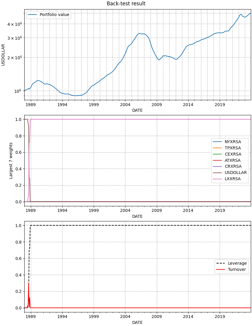
BACK-TEST RESULT OF MPO WITH HIGHEST (OUT-OF-SAMPLE) PROFIT
#################################################################
Universe size 21
Initial timestamp 1988-01-01 00:00:00+00:00
Final timestamp 2023-12-01 00:00:00+00:00
Number of periods 432
Initial value (USDOLLAR) 1.000e+06
Final value (USDOLLAR) 4.988e+06
Profit (USDOLLAR) 3.988e+06
Avg. return (annualized) 4.5%
Volatility (annualized) 3.6%
Avg. excess return (annualized) 1.5%
Avg. active return (annualized) 1.5%
Excess volatility (annualized) 3.7%
Active volatility (annualized) 3.7%
Avg. growth rate (annualized) 4.5%
Avg. excess growth rate (annualized) 1.4%
Avg. active growth rate (annualized) 1.4%
Avg. TransactionCost 1bp
Max. TransactionCost 300bp
Sharpe ratio 0.40
Information ratio 0.40
Avg. drawdown -12.1%
Min. drawdown -42.2%
Avg. leverage 97.8%
Max. leverage 100.1%
Avg. turnover 0.1%
Max. turnover 30.0%
Avg. policy time 0.011s
Avg. simulator time 0.005s
Of which: market data 0.001s
Total time 7.199s
#################################################################
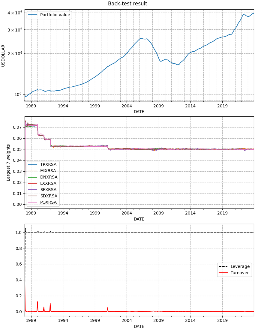
And these are the figure that are plotted.
The result of the cvxportfolio.Uniform policy, which allocates equal
weight to all non-cash assets: